


Investors holding Bitcoin alongside US stocks cannot tell whether their portfolio has become safer simply from a negative correlation between the assets’ price paths. A historical comparison through September 4 shows why: Bitcoin and the S&P 500 can move further apart over a year while still posting losses on many of the same trading dates.
Crypto asset manager Bitwise’s September 7 Market Compass described its 260-day correlation as the lowest since 2015. Its chart measures the logarithms of price levels. In CryptoSlate’s calculation using FRED data, that measure was about −0.62. Correlation between percentage returns over 260 common trading observations was +0.40.
The two figures measure different things. The first tracks how the two price paths moved over the period. The second tracks whether their percentage gains and losses tended to move together. Neither shows on its own that Bitcoin will offset losses when stocks fall.
The FRED prices are also recorded at different times of day. The comparison uses available daily observations, not simultaneous closing prices, so it cannot precisely measure how Bitcoin responds to an equity-market shock.
Two prices can diverge while losses overlap
Bitwise explicitly labels its chart as a log-level calculation and credits Bloomberg and Bitwise Europe. The calculation describes medium-term movement in the two price paths. It is not a daily-return statistic, nor should it be treated as a mistaken version of one.
For someone holding both assets, portfolio gains and losses depend on returns. A negative relationship between price levels does not guarantee negative covariance between returns. In simpler terms, two assets can drift in different directions over months while still rising or falling together on individual days. Their volatility and portfolio weights also determine how much that co-movement affects the portfolio.
The FRED Bitcoin observations and S&P 500 series show the difference. Using the last 260 common price dates through September 4 produces a log-level correlation of −0.6161. Using 260 percentage returns, from August 25, 2025, through September 4, 2026, produces +0.3957. Calculating 260 returns requires one additional starting price.
The negative log-level result resembles the trend in Bitwise’s report, but it is a proxy rather than an exact reproduction of its Bloomberg calculation. FRED’s public S&P history covers only 10 years, so it cannot independently establish the full “since 2015” ranking. That historical claim remains Bitwise’s.
The result also changes with the time period. In the same asynchronous data, return correlation was +0.14 over 30 observations, +0.32 over 60, +0.34 over 126 and +0.13 over 500, all ending September 4. Because those windows overlap, they are not independent evidence of a fixed long-term correlation.
A hypothetical portfolio shows what those differences can mean for an investor. Replacing 5% of the equity allocation with Bitcoin increased measured annualized volatility over the 260-return window, from 12.68% to 13.01%. The largest peak-to-trough decline also grew, from 9.10% to 9.98%.
Over 500 returns, the result reversed. The same Bitcoin allocation modestly reduced both measured volatility and maximum drawdown.
| Common-date return window | Allocation | Annualized volatility | Maximum drawdown |
|---|---|---|---|
| 260 observations | 100% S&P 500 | 12.68% | 9.10% |
| 260 observations | 95% S&P 500 / 5% Bitcoin | 13.01% | 9.98% |
| 500 observations | 100% S&P 500 | 16.11% | 18.90% |
| 500 observations | 95% S&P 500 / 5% Bitcoin | 15.73% | 18.66% |
Both windows end September 4, 2026. CryptoSlate calculations used the dated Bitcoin CSV and S&P 500 CSV, with weights reset at every common observation. Fees, taxes, and dividends were excluded. The S&P series is a price index, so these are not total investment-return comparisons. Maximum drawdown is the largest decline from a preceding portfolio peak within the sample.
The table uses prices recorded at different times rather than an executable strategy rebalanced at one shared closing time.
The two windows produced different results. Bitcoin increased measured volatility and drawdown in the 260-return sample, then modestly reduced both in the 500-return sample. A low correlation can diversify one source of risk without making a portfolio less volatile than equities alone.
What happened when equities fell
But full-period volatility is only part of the risk: investors also need to know what happened to Bitcoin when equities fell. The S&P 500 fell on 115 common dates across the 260-return sample. Bitcoin fell on 76 of them and averaged a 1.03% decline across all 115 equity-down observations. Correlation within that subset was +0.29.
Bitcoin fell even more consistently alongside stocks during larger declines. On the 25 observations when the S&P 500 fell more than 1%, Bitcoin declined on 22 and averaged a 2.59% loss. There were only three observations when equities fell more than 2%. Bitcoin fell on all three, averaging a 4.23% decline.
The results describe what happened in this sample, not what caused the moves. Three declines greater than 2% are also far too few to estimate how reliably Bitcoin would behave during a stock-market crash. Changing the window, loss threshold, or measurement time can substantially change results from such a small sample.
What the observations do show is that negative trend correlation coexisted with repeated losses in both assets. Investors cannot translate a chart of diverging price paths directly into an assumption that one holding will offset the other on a bad day.
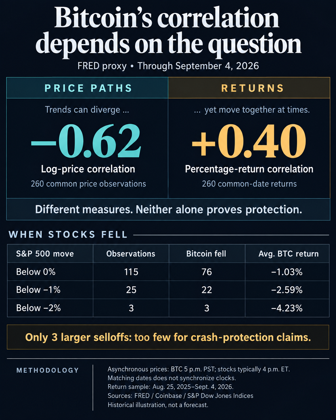
FRED records its Coinbase Bitcoin observation at 5 p.m. PST. Its S&P 500 observation represents the US market close, typically 4 p.m. ET. The two prices therefore share a calendar date but not a timestamp.
The calculations retain dates with valid observations for both assets, then measure changes between consecutive common dates. Bitcoin moves across intervening weekends or holidays are included in the interval. Stock prices are not filled forward to create additional trading observations.
The timing difference can change the result substantially. Moving Bitcoin’s observations back one calendar day changes the 260-return correlation to +0.14; moving them forward changes it to +0.03. Over 30 observations, those shifts produce −0.30 and −0.37, respectively.
Those shifts test possible lead-and-lag effects; they do not create synchronized prices. The sensitivity also means +0.40 should not be read as the exact correlation between Bitcoin and equities at the same moment. Measuring that would require prices recorded at matching times.
Bitwise also stops short of describing the decoupling as a hedge. Its report says a repeat of Bitcoin’s roughly 9,800% rise from mid-2015 to late 2017 is unlikely and warns that decouplings usually do not last.
For investors holding both assets, the numbers answer two separate questions. The negative log-level correlation shows that Bitcoin and the S&P 500 followed increasingly different price paths over the period. Their returns show that the two assets still lost money together on many of the same days.
Portfolio risk depends on the second question as well as allocation size, volatility, measurement time, and the period being studied.